Solving Gas Transmission PDEs using Koopman Operator Theory

Author: Yuan Li

The natural gas pipeline model is a nonlinear dynamic system driven by the boundary pressure and mass flow rate. Instead of solving the governing partial differential equations (PDEs) directly, we build a data-driven surrogate with Koopman operator theory and then use Solverz to perform multi-step prediction.

At each discrete time step \(k\), four signals are measured:

Signal	Role	Base value
\(P_\text{in}(k)\)	inlet pressure input	\(5\times10^6\) Pa
\(P_\text{out}(k)\)	outlet pressure output	\(5\times10^6\) Pa
\(m_\text{in}(k)\)	inlet mass flow input	\(10\) kg/s
\(m_\text{out}(k)\)	outlet mass flow output	\(10\) kg/s

All signals are normalized by their base values. The dataset contains \(N=1000\) samples, with the first \(N_\text{train}=700\) samples used for regression and the remaining ones used for prediction.

Observable Space

We define the lifted observable vector as

(1)\[\begin{split}\boldsymbol{\psi}(k)= \begin{bmatrix} P_\text{out}(k)\\ m_\text{out}(k)\\ \qty(-P_\text{out}(k))e^{-P_\text{out}(k)}\\ e^{-P_\text{out}(k)}\sin\qty(-P_\text{out}(k)) \end{bmatrix}\in\mathbb{R}^4.\end{split}\]

The first two entries are linear observables and the last two entries are nonlinear lifting terms used to capture the gas-flow dynamics.

Koopman Regression

Let \(\mathbf{X}\in\mathbb{R}^{N\times4}\) collect the observables and \(\mathbf{U}\in\mathbb{R}^{N\times2}\) collect the normalized inputs. The Koopman model is written as

(2)\[\boldsymbol{\psi}(k)=K_x\boldsymbol{\psi}(k-1)+K_u\mathbf{u}(k),\]

where \(K_x\in\mathbb{R}^{4\times4}\) and \(K_u\in\mathbb{R}^{4\times2}\) are constant matrices identified from training data.

Define the regression matrix over the training window as

(3)\[Z=\qty[\mathbf{X}_{0:T-1},\;\mathbf{U}_{1:T}]\in\mathbb{R}^{(T-1)\times6},\]

then the least-squares solution is

\[\begin{bmatrix}K_x\mid K_u\end{bmatrix}^{\mathsf{T}}=Z^\dagger \mathbf{X}_{1:T}.\]

Solverz Formulation

To run multi-step prediction in Solverz, we rewrite (2) into a residual equation for each state component:

(4)\[F_i\bigl(\mathbf{x}(k),\mathbf{x}(k-1),\mathbf{u}(k)\bigr) =x_i(k)-\sum_{j=0}^{3}K_x[i,j]x_j(k-1)-K_u[i,0]u_P(k)-K_u[i,1]u_M(k)=0,\]

for \(i=0,\ldots,3\), where \(\mathbf{x}(k)\equiv\boldsymbol{\psi}(k)\).

The delayed state \(\mathbf{x}(k-1)\) is represented by AliasVar, so Solverz can automatically substitute the state value from the previous time step.

The complete implementation is shown below. The source file and the lightweight benchmark data package are stored in the same directory on GitHub.

import os

import matplotlib.pyplot as plt
import numpy as np

from Solverz import Eqn, Model, Opt, TimeSeriesParam, Var, fdae_solver, made_numerical
from Solverz.variable.ssymbol import AliasVar

current_dir = os.getcwd()
data_path = os.path.join(current_dir, "test_koopman", "koopman_data.npz")

BASEVALUE_P = 5e6
BASEVALUE_M = 10.0
N_TRAIN = 700
N_TEST = 300
N = N_TRAIN + N_TEST
DT = 1.0

# %% Load dataset
data = np.load(data_path)
pin_norm = data["pin"]
pout_norm = data["pout"]
qin_norm = data["qin"]
qout_norm = data["qout"]

# %% Build observables
x_data = np.column_stack(
    [
        pout_norm,
        qout_norm,
        (-pout_norm) * np.exp(-pout_norm),
        np.exp(-pout_norm) * np.sin(-pout_norm),
    ]
)
u_data = np.column_stack([pin_norm, qin_norm])

# %% Koopman regression
z_reg = np.hstack([x_data[: N_TRAIN - 1], u_data[1:N_TRAIN]])
k_all = (np.linalg.pinv(z_reg) @ x_data[1:N_TRAIN]).T
kx = k_all[:, :4]
ku = k_all[:, 4:]

# %% Solverz rollout
x0_test = x_data[N_TRAIN]
u_future = u_data[N_TRAIN + 1 :]
t_pred = len(u_future)
t_series = np.arange(t_pred + 1, dtype=float) * DT
u_p_series = np.concatenate([[u_future[0, 0]], u_future[:, 0]])
u_m_series = np.concatenate([[u_future[0, 1]], u_future[:, 1]])

model = Model()
model.x = Var("x", value=x0_test)
model.x_prev = AliasVar("x", step=1, value=x0_test)
model.u_P = TimeSeriesParam("u_P", v_series=u_p_series, time_series=t_series)
model.u_M = TimeSeriesParam("u_M", v_series=u_m_series, time_series=t_series)

for i in range(4):
    kx_row_sum = sum(kx[i, j] * model.x_prev[j] for j in range(4))
    ku_u = ku[i, 0] * model.u_P + ku[i, 1] * model.u_M
    model.__dict__[f"eq_{i}"] = Eqn(f"eq_{i}", model.x[i] - kx_row_sum - ku_u)

symbolic_model, y0 = model.create_instance()
numerical_model = made_numerical(symbolic_model, y0, sparse=True)
sol = fdae_solver(numerical_model, [0, t_pred * DT], y0, Opt(step_size=DT, pbar=False))
x_pred = sol.Y["x"]

# %% Plot
x_true = x_data[N_TRAIN : N_TRAIN + len(x_pred)]
rmse = np.sqrt(np.mean((x_true - x_pred) ** 2))

obs_labels = ["Pout linear", "Mout linear", "-Pout exp(-Pout)", "exp(-Pout) sin(-Pout)"]
t_all = np.arange(N)
t_pred_idx = np.arange(N_TRAIN, N_TRAIN + len(x_pred))

fig, axes = plt.subplots(4, 1, figsize=(12, 12), sharex=True)
for idx, ax in enumerate(axes):
    ax.plot(t_all, x_data[:, idx], "k-", lw=1.5, label="True value")
    ax.plot(t_pred_idx, x_pred[:, idx], "r--", lw=1.5, label="Prediction")
    ax.axvline(N_TRAIN, color="g", ls="-.", lw=1.5, label="Train/test boundary")
    ax.set_ylabel(obs_labels[idx])
    ax.grid(alpha=0.3)
    ax.legend(fontsize=8, loc="best")

axes[-1].set_xlabel("Time step k")
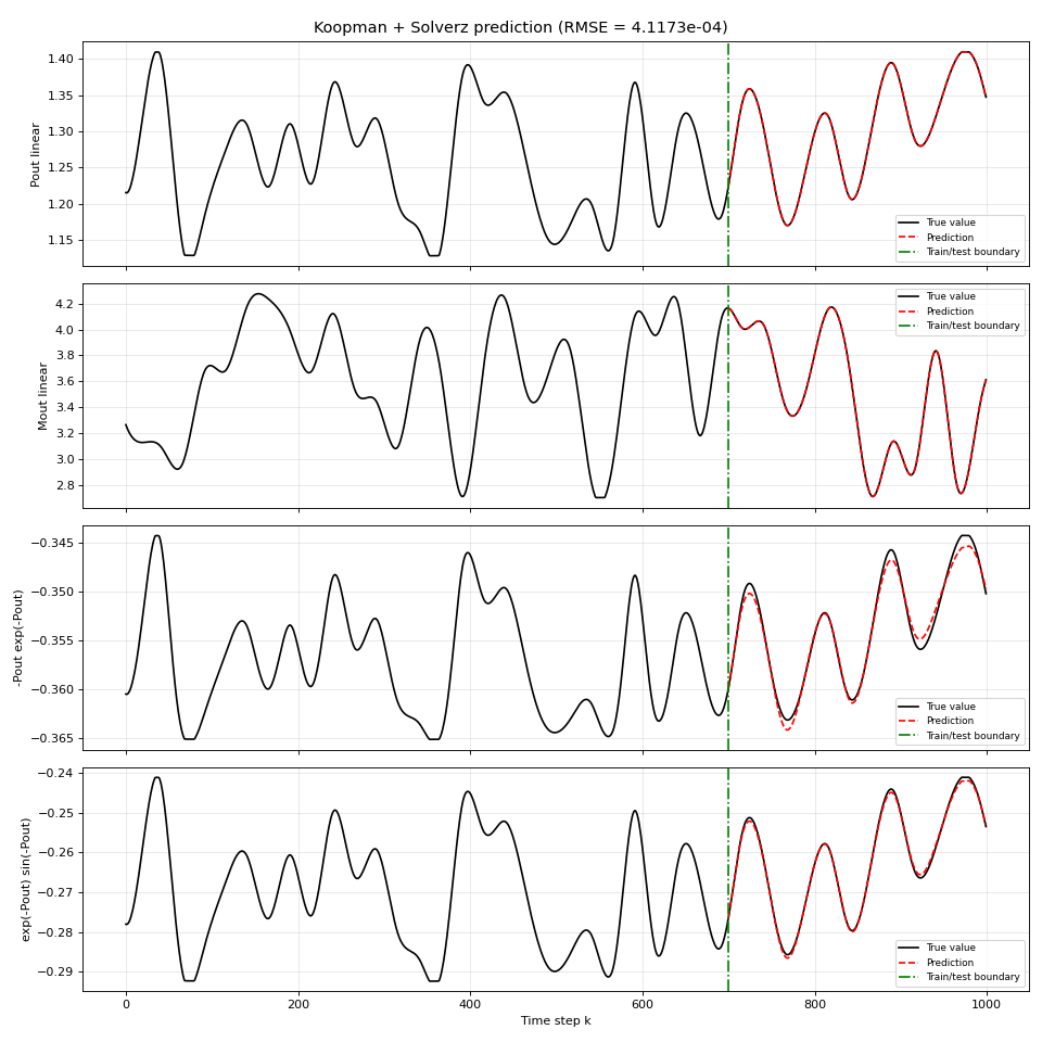
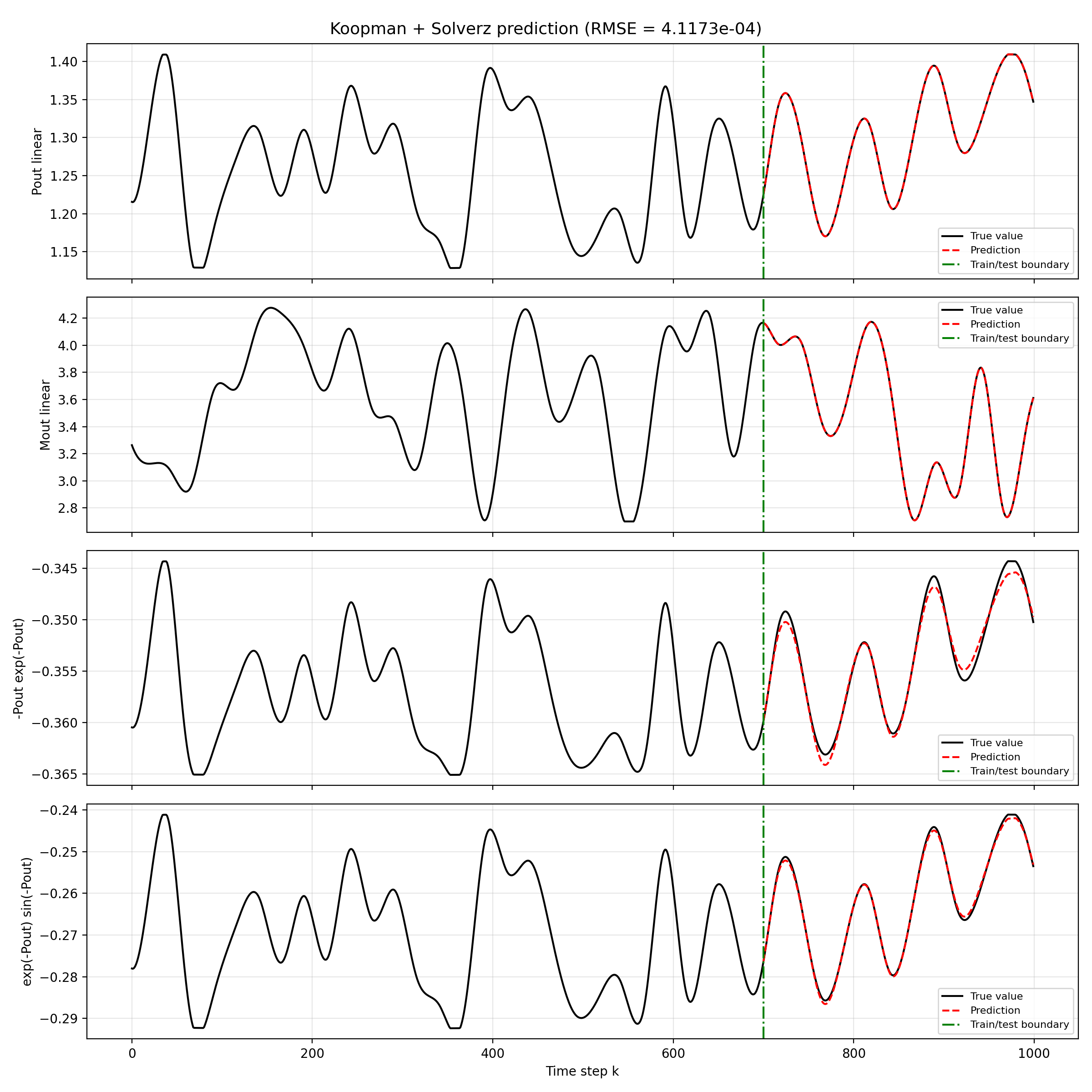
fig.suptitle(f"Koopman + Solverz prediction (RMSE = {rmse:.4e})", fontsize=13)
plt.tight_layout()
plt.show()

The prediction result is

(Source code, png, hires.png, pdf)

The learned Koopman model tracks the test trajectory well, and the plotted curves show that the Solverz rollout reproduces the main trends of all lifted observables.