Solving Gas Transmission PDEs using Characteristics
Author: Ruizhi Yu
The hyperbolic partial differential equations (PDEs) describing the conservation of isothermal gas transmission are
where
\(p\) is the spatial and temporal distribution of pressure
\(q\) is the spatial and temporal distribution of mass flow,
\(c\) is the sound velocity,
\(S\) is the pipe cross-sectional area,
\(\lambda\) is the friction coefficient,
\(D\) is the pipe diameter,
Suppose we have, for a pipe with length \(L\), the initial conditions
and the boundary conditions
we use the method of characteristics to solve solutions of the above PDEs numerically.
Rewrite (1) as
wherein the matrix can be diagonalized as
Multiplying \(P^{-1}\) to both sides of (2), we have
which can also be written as the total derivative forms with formulae
and
Multiplying \(\dd t\) to both sides of (3), we have
which holds only along the characteristic \(\dd x/\dd t=c\).
Similarly, we have, along the characteristic \(\dd x/\dd t=-c\),
Given difference stencil
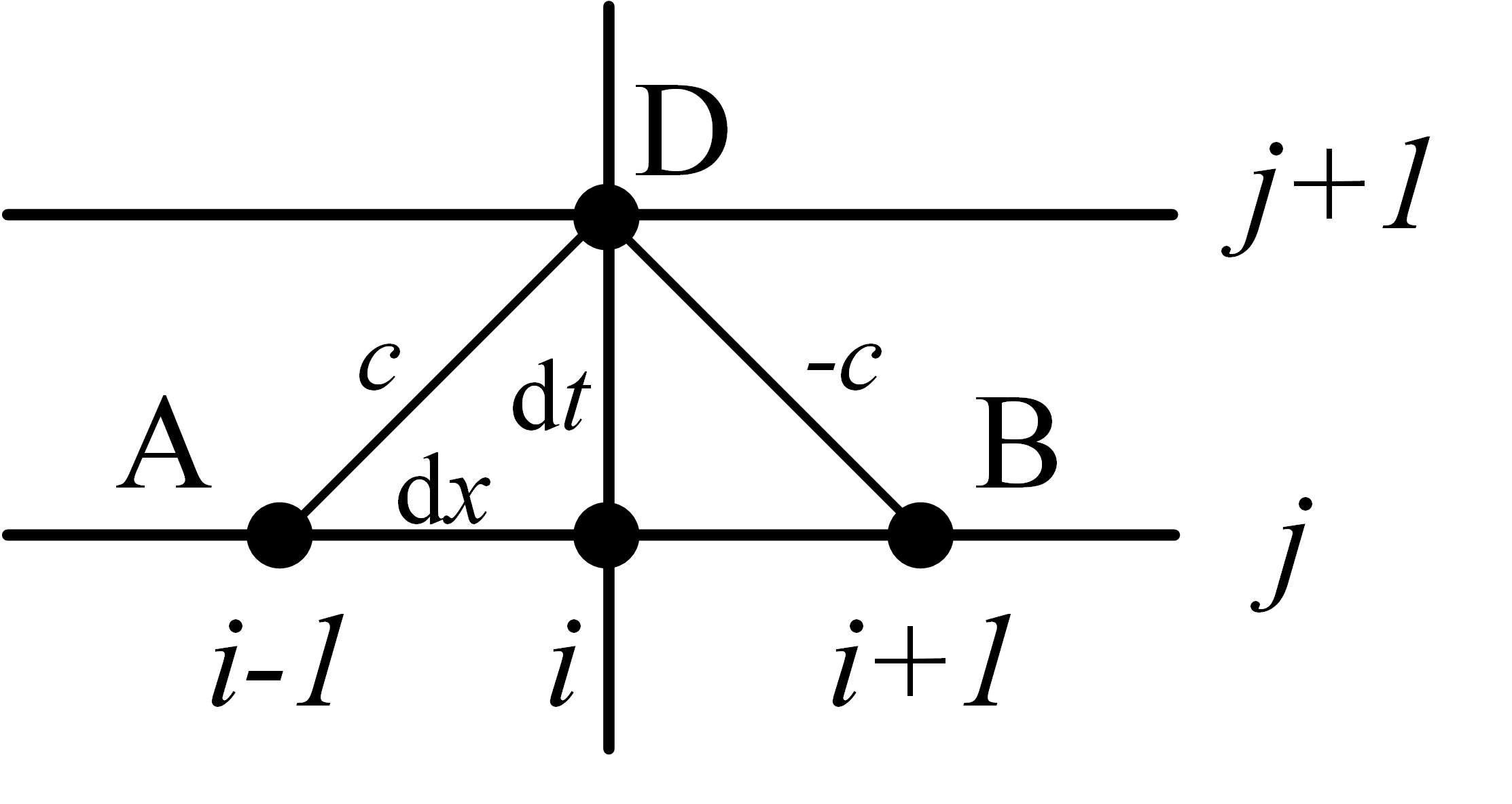
we can integrate (4) along A to D, and approximate the \(q|q|/p\) term by \((q_A+q_D)|q_A+q_D|/(p_A+p_D)\).
Then we obtain
Similarly,
If we divided the total pipe length into \(M\) sections, we finally have the finite difference algebraic equations
The following codes are the Solverz implementation of the characteristics.
import matplotlib.pyplot as plt
import numpy as np
from sympy import Integer
from Solverz import (Var, Param, Eqn, Opt, Abs,
made_numerical, TimeSeriesParam, Model, AliasVar, fdae_solver)
# %% mdl
L = 51000 * 0.8
p0 = 6621246.69079594
q0 = 14
va = Integer(340)
D = 0.5901
S = np.pi * (D / 2) ** 2
lam = 0.03
dx = 500
dt = 1.4706
M = int(L / dx)
m1 = Model()
m1.p = Var('p', value=p0 * np.ones((M + 1,)))
m1.q = Var('q', value=q0 * np.ones((M + 1,)))
m1.p0 = AliasVar('p', init=m1.p)
m1.q0 = AliasVar('q', init=m1.q)
m1.ae1 = Eqn('cha1',
m1.p[1:M + 1] - m1.p0[0:M] + va / S * (m1.q[1:M + 1] - m1.q0[0:M]) +
lam * va ** 2 * dx / (4 * D * S ** 2) * (m1.q[1:M + 1] + m1.q0[0:M]) * Abs(m1.q[1:M + 1] + m1.q0[0:M]) / (
m1.p[1:M + 1] + m1.p0[0:M]))
m1.ae2 = Eqn('cha2',
m1.p0[1:M + 1] - m1.p[0:M] + va / S * (m1.q[0:M] - m1.q0[1:M + 1]) +
lam * va ** 2 * dx / (4 * D * S ** 2) * (m1.q[0:M] + m1.q0[1:M + 1]) * Abs(m1.q[0:M] + m1.q0[1:M + 1]) / (
m1.p[0:M] + m1.p0[1:M + 1]))
T = 5 * 3600
pb1 = 1e6
pb0 = 6621246.69079594
pb_t = [pb0, pb0, pb1, pb1]
tseries = [0, 1000, 1000 + 10 * dt, T]
m1.pb = TimeSeriesParam('pb',
v_series=pb_t,
time_series=tseries)
m1.qb = Param('qb', q0)
m1.bd1 = Eqn('bd1', m1.p[0] - m1.pb)
m1.bd2 = Eqn('bd2', m1.q[M] - m1.qb)
fdae, y0 = m1.create_instance()
nfdae, code = made_numerical(fdae, y0, sparse=True, output_code=True)
# %% solution
sol = fdae_solver(nfdae, [0, T], y0, Opt(step_size=dt))
# %% visualize
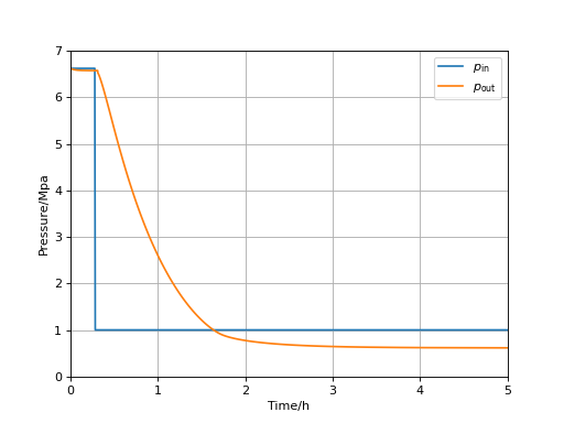
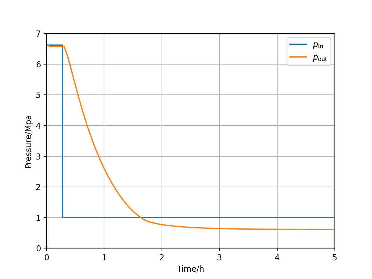
plt.plot(sol.T / 3600, sol.Y['p'][:, 0] / 1e6, label=r'$p_\text{in}$')
plt.plot(sol.T / 3600, sol.Y['p'][:, -1] / 1e6, label=r'$p_\text{out}$')
plt.xlim([0, 5])
plt.ylim([0, 7])
plt.xlabel('Time/h')
plt.ylabel('Pressure/Mpa')
plt.legend()
plt.grid()
plt.show()
Finally, we have
(Source code, png, hires.png, pdf)
