Method-of-Lines Solution of Network Gas Flow

Author: Ruizhi Yu

Here we consider the transmission of gas in the following networks.

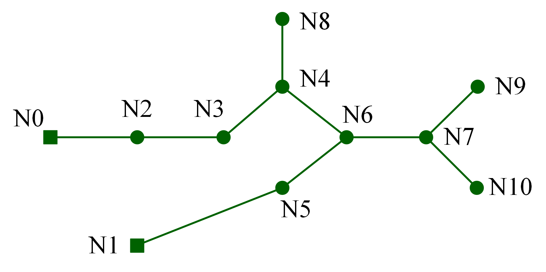
The squares are the sources producing gas while the circles are the consumers. The edges denote the pipes in which the gas is transferred. To get an insight into the state transfer of pressure and mass flow, we follow the derivations by Professor Gerd Steinebach[1] which is based on the method-of-lines.

Modelling

Gas Pipes

First, we have, for each pipe, the PDEs describing the isothermal gas transmission, with formulae

(1)\[\begin{split}\pdv{p}{t}+\frac{c^2}{S}\pdv{q}{x}=&0,\\ \pdv{q}{t}+S\pdv{p}{x}+\frac{\lambda c^2q|q|}{2DSp}=&0\end{split}\]

where

• \(p\) is the spatial and temporal distribution of pressure

• \(q\) is the spatial and temporal distribution of mass flow

• \(c\) is the sound velocity

• \(S\) is the pipe cross-sectional area

• \(\lambda\) is the friction coefficient,

• \(D\) is the pipe diameter,

and, suppose we have a pipe with length \(L\), the initial conditions

\[p(x, 0)=p_0,\quad q(x,0)=q_0,\]

and the boundary conditions

\[p(0, t)=p_\text{b}(t),\quad q(L,t)=q_\text{b}(t).\]

Network Constraints

Then there come the network constraints, that is,

the continuity of mass flow

\[\sum_{i\in \mathbb{E}^\text{in}_k} q_i^\text{in}-\sum_{j\in \mathbb{E}^\text{out}_k} q_j^\text{out}=q_k, \quad k\in \mathbb{V}\]

where \(q_i^\text{in/out}\) is the inlet/outlet mass flow of pipe \(i\). \(\mathbb{E}_k^\text{in/out}\) is the set of edges flowing into/out of node \(k\). \(q_k\) is the injection mass flow of node \(k\),

and the continuity of pressure

\[p_k=p^\text{out}_i=p^\text{in}_j,\quad i\in\mathbb{E}_k^\text{out},\ j\in\mathbb{E}_k^\text{in},\]

where \(p_k\) is the pressure of node \(k\), \(p_i^\text{in/out}\) is the inlet/outlet pressure of pipe \(i\).

Solution

The Method of Lines

The method of lines does the semidiscretization of PDEs for a system of ODEs. First, the PDE systems (1) are summarized by

\[ \pdv{u}{t}+\pdv{f(u)}{x}=S(u), \quad x\in [0, L]. \label{hyperbolicpde}\]

with state vector \(u\), flux function \(f(u)\) and source term \(S(u)\). The space interval is discretized into \(0=x_0<x_1<\cdots<x_{M-1}<x_M=L\) with constant step size \(\Delta x=x_{j+1}-x_{j}\).

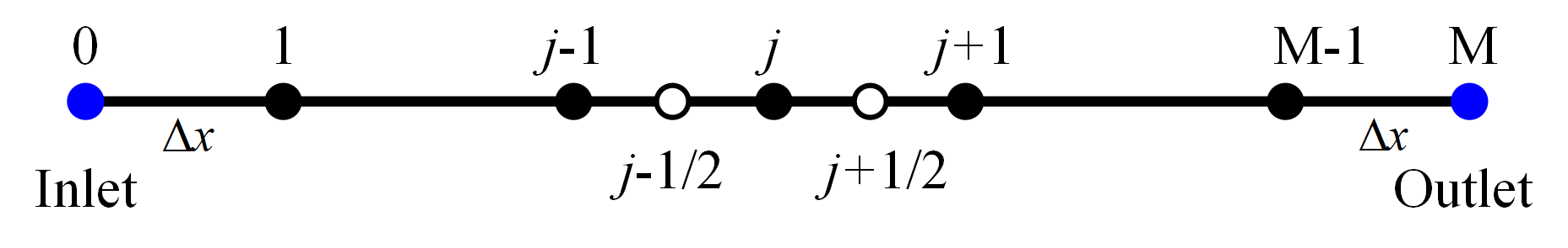
The space derivatives are approximated by \(\pdv{f(u)}{x}=\frac{f_{i+1/2}-f_{i-1/2}}{\Delta x}\) with suitable chosen flux values \(f_{i\pm 1/2}\) leading to the semi-discretized system of ODEs

\[ \dv{u_j}{t}+\frac{f_{j+1/2}-f_{j-1/2}}{\Delta x}=S(u_j), \quad j=1,\cdots,M-1.\]

The methods to get stable discretizations have been well studied. Here, a local Lax-Friedrichs approach is applied:

\[f_{j+1 / 2}=\frac{1}{2}\left(f_{j+1 / 2}^{+}+f_{j+1 / 2}^{-}-\left|\lambda_{j+1 / 2}\right|\left(u_{j+1 / 2}^{+}-u_{j+1 / 2}^{-}\right)\right).\]

We put

\[\lambda_{j+1/2}=\rho\qty(\dv{f}{x})\]

where \(\rho\) is the spectral radius of \(\dv{f}{x}\). In the above case, it would be \(c\) since

\[\begin{split}A\triangleq \pdv{f(u)}{x}= \begin{bmatrix} \boldsymbol{0}&\frac{c^2}{S}\\ S&\boldsymbol{0} \end{bmatrix},\end{split}\]

\[|\lambda I-A|=\lambda^2 - c^2=0,\]

and

\[\lambda =\pm c.\]

We would recommend the books of Professor Hirsch[2] and Professor Bertoluzza[3] for detailed derivation. However, we found that in the linear case, to set \(\lambda_{j+1/2}\) lowers the accuracy. We can just put \(\lambda_{j+1/2}=0\) here.

The first order discretization is given by the choice

\[f_{j+1/2}^+=f(u_{j+1}),\quad f_{j+1/2}^-=f(u_j), \quad, u_{j+1 / 2}^{+}=u_{j+1}, \quad, u_{j+1 / 2}^{-}=u_{j}, \quad j=1,\cdots,M-1.\]

\(f_{j-1/2}\) can be obatined by moving the stencil one \(\Delta x\) left. Higher order can be achieved by the Kurganov-Tadmor[4] or the WENO method[5].

Numerical Boundaries

The above semi-discretization uses a three-point stencil. However, for \(p\) and \(q\) at the boundary, i.e., \(p_M\) and \(q_0\), we ought to derive the numerical boundaries, which are algebraic equations, to finally complement the equations.

Perform the eigendecomposition of \(A\), we have

\[A v=v\Lambda.\]

Hence, we have

\[v^{-1}\pdv{u}{t}+\Lambda v^{-1}\pdv{u}{x}=v^{-1}S(u),\]

where

\[\begin{split}v^{-1}= \begin{bmatrix} \frac{S}{2c}&\frac{1}{2}\\ -\frac{S}{2c}&\frac{1}{2} \end{bmatrix}\ \text{and}\ \Lambda= \begin{bmatrix} c&0\\ 0&-c \end{bmatrix}.\end{split}\]

Letting

\[\begin{split}\delta w=v^{-1}\delta u=\begin{bmatrix} \frac{S}{2c}\delta p+\frac{1}{2}\delta q\\ -\frac{S}{2c}\delta p+\frac{1}{2}\delta q \end{bmatrix}\end{split}\]

we have

\[\pdv{w}{t}+\Lambda\pdv{w}{x}=v^{-1}S(u).\]

Neglecting the source term, we have

\[\dv{w}{t}=0.\]

That is, Riemann variable \(w_1\) is invariant along the path line \(\dv*{x}{t}=c\) and \(w_2\) is invariant along the path line \(\dv*{x}{t}=-c\).

Two characteristics are defined as

\[\begin{split}\begin{aligned} \text{On}\ C_+\text{:}\quad& \dv{x}{t}=c,\\ \text{On}\ C_-\text{:}\quad& \dv{x}{t}=-c. \end{aligned}\end{split}\]

Integrating \(w_1\) along \(c_+\), we have

\[w_1=\int\frac{S}{2c}\delta p+\int\frac{1}{2}\delta q=\frac{S}{2c}p+\frac{1}{2}q.\]

Similarly,

\[w_2=-\frac{S}{2c}p+\frac{1}{2}q.\]

To obtain the right numerical boundary condition, we have to use the invariant \(\frac{S}{2c}p+\frac{1}{2}q\) along \(C_+\) for its pointing to the right boundary.

Letting

\[S p+c q\triangleq I_M(x,t),\]

we have

\[ I_M(x_M,t_1)= I_M(x_{M-1},t)\quad \text{where}\quad t_1=\frac{\Delta x}{c}+t,\]

\[ I_M(x_M,t_2)= I_M(x_{M-2},t)\quad \text{where}\quad t_2=\frac{2\Delta x}{c}+t.\]

By linear extrapolation, we have

\[ I_M(x_\text{M},t)=\frac{ I_M(x_M,t_2)- I_M(x_M,t_1)}{t_2-t_1}(t-t_1)+ I_M(x_M,t_1)= 2 I_M(x_{M-1},t)- I_M(x_{M-2},t). \]

Similarly, we have

\[ I_0(x_0,t)= 2I_0(x_1,t)-I_0(x_2,t). \]

Finally, we have numerical boundary conditions, for \(p_M\),

\[ p_M+\frac{c}{S} q_M+\qty( p_{M-2}+\frac{c}{S} q_{M-2})-2\qty( p_{M-1}+\frac{c}{S} q_{M-1})=0.\]

Similarly, we have, for \(q_0\),

\[\qty(\frac{S}{c} p_2- q_2)+\frac{S}{c} p_0- q_0-2\qty(\frac{S}{c} p_1- q_1)=0.\]

Implementation in Solverz

Here presents the Solverz implementation of method-of-lines with respect to the gas network at the very beginning. The data for initialization, the steady_gas_flow_model.pkl, can be found in related directory of the source repo.

We want to see the impacts of source pressure increase, so we set Piset0 as a TimeSeriesParam.

import numpy as np
import pandas as pd
import os
import networkx as nx

from Solverz import load, Eqn, Ode, Abs, Model, Var, Param, TimeSeriesParam, made_numerical, Rodas, Opt
import matplotlib.pyplot as plt

# %%
# create G of the network using networkx
idx_pipe = np.arange(10)
idx_node = np.arange(11)
idx_from = [0, 3, 1, 4, 4, 5, 7, 7, 2, 6]
idx_to = [2, 4, 5, 8, 6, 6, 9, 10, 3, 7]

G = nx.DiGraph()

for i in range(len(idx_pipe)):
    G.add_node(idx_from[i])
    G.add_node(idx_to[i])
    G.add_edge(idx_from[i], idx_to[i], idx=idx_pipe[i])
A = nx.incidence_matrix(G,
                        nodelist=idx_node,
                        edgelist=sorted(G.edges(data=True), key=lambda edge: edge[2].get('idx', 1)),
                        oriented=True)

# %%
m = Model()
Piv = np.array([10., 8., 9.25356807, 8.44138875, 7.54225206,
                7.67010339, 7.32536498, 6.09107411, 7.27354882, 5.56663968,
                5.87805022]) * 1e6
m.Pi = Var('Pi', value=Piv)  # node pressure
f = np.array([39.57682738, 39.57682738, 23.73641444, 20.83, 18.74682738,
              23.73641444, 25.81324182, 16.67, 39.57682738, 42.48324182])
m.qn = Var('qn', value=A @ f)  # node injection mass flow
va = 340
m.D = Param('D', value=0.5 * np.ones(10))
m.Area = Param('Area', np.pi * (m.D.value / 2) ** 2)
m.lam = Param('lam', value=0.03 * np.ones(10))
Piset0 = 10e6
m.Piset0 = TimeSeriesParam('Piset0',
                           v_series=[Piset0, Piset0 + 0.5e6, Piset0 + 0.5e6],
                           time_series=[0, 2 * 3600, 10 * 3600])
m.Piset1 = Param('Piset1', value=8e6)
L = 51000*np.ones(10)
dx = 100
M = np.floor(L / dx).astype(int)
for j in range(10):
    p0 = np.linspace(Piv[idx_from[j]], Piv[idx_to[j]], M[j] + 1)
    m.__dict__['p' + str(j)] = Var('p' + str(j), value=p0)
    m.__dict__['q' + str(j)] = Var('q' + str(j), value=f[j] * np.ones(M[j] + 1))

# % method of lines
for node in G.nodes:
    eqn_q = m.qn[node]
    for edge in G.in_edges(node, data=True):
        pipe = edge[2]['idx']
        idx = str(pipe)
        qi = m.__dict__['q' + idx]
        pi = m.__dict__['p' + idx]
        eqn_q = eqn_q - qi[M[pipe]]
        m.__dict__[f'pressure_outlet_pipe{idx}'] = Eqn(f'Pressure node {node} pipe {idx} outlet',
                                                       m.Pi[node] - pi[M[pipe]])

    for edge in G.out_edges(node, data=True):
        pipe = edge[2]['idx']
        idx = str(pipe)
        qi = m.__dict__['q' + idx]
        pi = m.__dict__['p' + idx]
        eqn_q = eqn_q + qi[0]
        m.__dict__[f'pressure_inlet_pipe{idx}'] = Eqn(f'Pressure node {node} pipe {idx} inlet',
                                                      m.Pi[node] - pi[0])

    m.__dict__[f'mass_continuity_node{node}'] = Eqn('mass flow continuity of node {}'.format(node), eqn_q)

m.Pressure_source_node0 = Eqn('Pressure of source node0',
                              m.Pi[0] - m.Piset0)
m.Pressure_source_node1 = Eqn('Pressure of source node1',
                              m.Pi[1] - m.Piset1)
m.mass_injection_ns_nodes = Eqn('Mass flow injection of non-source node',
                                m.qn[2:8])
m.mass_injection_node8 = Eqn('Mass flow injection of node 8',
                             m.qn[8] - 20.83)
m.mass_injection_node9 = Eqn('Mass flow injection of node 9',
                             m.qn[9] - 18.81898528)
m.mass_injection_node10 = Eqn('Mass flow injection of node 10',
                              m.qn[10] - 15.12876112)


def mol_tvd1_p_eqn_rhs1(P_list, Q_list, S, va, dx):
    P_list = [arg.symbol if isinstance(arg, Var) else arg for arg in P_list]
    Q_list = [arg.symbol if isinstance(arg, Var) else arg for arg in Q_list]
    pm1, p0, pp1 = P_list
    qm1, q0, qp1 = Q_list
    # return -va ** 2 / S * (qp1 - qm1) / (2 * dx) + va * (pp1 - 2 * p0 + pm1) / (2 * dx)
    return -va ** 2 / S * (qp1 - qm1) / (2 * dx)


def mol_tvd1_q_eqn_rhs1(P_list, Q_list, S, va, lam, D, dx):
    P_list = [arg.symbol if isinstance(arg, Var) else arg for arg in P_list]
    Q_list = [arg.symbol if isinstance(arg, Var) else arg for arg in Q_list]
    pm1, p0, pp1 = P_list
    qm1, q0, qp1 = Q_list
    # return -S * (pp1 - pm1) / (2 * dx) + va * (qp1 - 2 * q0 + qm1) / (2 * dx) - lam * va ** 2 * q0 * Abs(q0) / (
    #         2 * D * S * p0)
    return -S * (pp1 - pm1) / (2 * dx) - lam * va ** 2 * q0 * Abs(q0) / (
            2 * D * S * p0)


# method of lines
p_list = []
q_list = []
for edge in G.edges(data=True):
    f_node = edge[0]
    t_node = edge[1]
    j = edge[2]['idx']
    Mj = M[j]
    pj = m.__dict__['p' + str(j)]
    qj = m.__dict__['q' + str(j)]
    Dj = m.D[j]
    Sj = m.Area[j]
    lamj = m.lam[j]

    rhs = mol_tvd1_q_eqn_rhs1([pj[0:Mj - 1], pj[1:Mj], pj[2:Mj + 1]],
                              [qj[0:Mj - 1], qj[1:Mj], qj[2:Mj + 1]],
                              Sj,
                              va,
                              lamj,
                              Dj,
                              dx)
    m.__dict__['q' + str(j) + '_eqn2'] = Ode(f'weno3-q{j}2',
                                             rhs,
                                             qj[1:Mj])

    rhs = mol_tvd1_p_eqn_rhs1([pj[0:Mj - 1], pj[1:Mj], pj[2:Mj + 1]],
                              [qj[0:Mj - 1], qj[1:Mj], qj[2:Mj + 1]],
                              Sj,
                              va,
                              dx)
    m.__dict__['p' + str(j) + '_eqn3'] = Ode(f'weno3-p{j}3',
                                             rhs,
                                             pj[1:Mj])

    m.__dict__['p' + str(j) + 'bd1'] = Eqn(pj.name + 'bd1',
                                           Sj * pj[Mj] + va * qj[Mj] + Sj * pj[Mj - 2] + va * qj[
                                               Mj - 2] - 2 * (
                                                   Sj * pj[Mj - 1] + va * qj[Mj - 1]))
    m.__dict__['q' + str(j) + 'bd2'] = Eqn(qj.name + 'bd2',
                                           Sj * pj[2] - va * qj[2] + Sj * pj[0] - va * qj[0] - 2 * (
                                                   Sj * pj[1] - va * qj[1]))

# %% initialize m
sdae, y0 = m.create_instance()
ndae, code = made_numerical(sdae, y0, sparse=True, output_code=True)

sol = Rodas(ndae,
            [0, 3600 * 50],
            y0)

# %% visualize
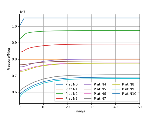
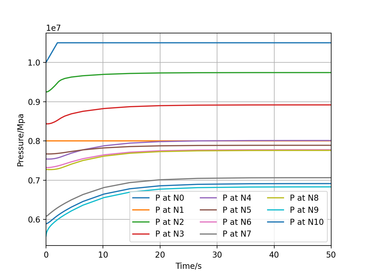
plt.plot(sol.T / 3600, sol.Y['Pi'], label=[f'P at N{i}' for i in range(11)])
plt.xlim([0, 50])
plt.xlabel('Time/s')
plt.ylabel(r'Pressure/Mpa')
plt.legend(ncols=3)
plt.grid()
plt.show()

We illustrate the variation of node pressure as follows.

(Source code, png, hires.png, pdf)

---

[1]

Steinebach, G., Dreistadt, D.M. (2021). Water and Hydrogen Flow in Networks: Modelling and Numerical Solution by ROW Methods. In: Jax, T., Bartel, A., Ehrhardt, M., Günther, M., Steinebach, G. (eds) Rosenbrock—Wanner–Type Methods. Mathematics Online First Collections. Springer, Cham. https://doi.org/10.1007/978-3-030-76810-2_2

[2]

C. Hirsch, Numerical Computation of Internal and External Flows, Volume 2: Computational Methods for Inviscid and Viscous Flows. West Sussex, England: John Wiley & Sons, 1990.

[3]

Silvia Bertoluzza, Giovanni Russo, Silvia Falletta, Chi-Wang Shu (2009). Numerical Solutions of Partial Differential Equations. Birkhäuser Basel. https://doi.org/10.1007/978-3-7643-8940-6

[4]

Alexander Kurganov, Eitan Tadmor, New High-Resolution Central Schemes for Nonlinear Conservation Laws and Convection–Diffusion Equations, Journal of Computational Physics, Volume 160, Issue 1, 2000, Pages 241-282, https://doi.org/10.1006/jcph.2000.6459

[5]

C.-W. Shu, “Essentially non-oscillatory and weighted essentially non- oscillatory schemes for hyperbolic conservation laws,” in Advanced Numerical Approximation of Nonlinear Hyperbolic Equations: Lectures given at the 2nd Session of the Centro Internazionale Matematico Estivo (C.I.M.E.) held in Cetraro, Italy, June 23–28, 1997, A. Quarteroni, Ed. Berlin, Heidelberg: Springer Berlin Heidelberg, 1998, pp. 325–432.